In this blog, we will review how Perceiver AI performs in finding solutions as compared to other data science tools, specifically, the solution for the sum of n numbers problem. We will compare Perceiver against TensorFlow, a deep learning software library for machine learning and AI applications, to see how the two techniques perform with respect to the accuracy and scalability of the models they create. To watch the demonstration video, please click here.

Input Review

We’ll start by reviewing the input for our comparison.

1. We are using a Comma Separated Values (CSV) file where we have an output column $SUM which is the sum of the first $VAR1 numbers. The format of the CSV file is described in the Training Set image below.

2. We are also injecting spurious variables in the dataset, including some that are somewhat correlated in some sectors, but their purpose is to deceive the training process. These are $VAR2-$VAR7 & $PARAM2.

Training Set (First 29 of 49 rows displayed)

We take the first 49 rows and make it the training set for TensorFlow. Then, we split out the last 11 records and make it the test set. These last several rows in the test set are a set of inputs that are farther away from the training set to compare how the two methods perform.

Test Set

Using TensorFlow to Predict the Sum of n Numbers

Next, let’s take a look at our TensorFlow code. We’re importing all of our libraries; this is a deep learning model using Keras, which is a standard library utilized by many deep learning solutions. We have a deep learning model with two hidden layers of 64 variables. It’s a very common practice to use a power of the input variables, which in this case is 8.

A Portion of the Keras code

We have a dense output layer that’s intended to help with the end result of some of the numbers. We will read the two files, the training set and the test set, and drop variables into input training and output training and input test and output test files. Then we build a model. What happens next is as follows: once the model is trained for a thousand epochs, we then predict the training set, which should always be accurate. After that, we’ll try to predict the test set, which wasn’t used during the training, to see how it performs.

In setting up this demonstration, we were a bit devious in that we split the test set with the variables farther away, using nontypical variables from the ones we used with the training set. While this might seem a little unfair, we used the same setup with Perceiver to see how it performs under similar circumstances.

When we ran this model in TensorFlow to see how it did, we found that it ran through the data and got to a RMSE of about 0.27, which is quite good, basically a rounding error. This is where TensorFlow performs quite well. It took all these input variables into the model and created something locally very accurate.

In summary, when it predicted the training set, the output values and the expected values were very close to what the network had predicted. But as we go to the test set, which contains values located farther away, we find that the errors become very large. The farther away it gets from the training set, the larger the errors become in terms of the difference between what we expect and what is produced.

TensorFlow Results

We encounter three issues: First, TensorFlow requires a tremendous amount of input to produce an accurate model across the entire range. Second, we can’t see the model anymore, we only have weights applied to these sets of layers, which cannot be interpreted as a formula. Third, nontypical inputs, being a much more complex model, will produce results that are outside of what’s expected. In such a situation, this could in some cases be considered as overfitting.

Using Perceiver to Predict the Sum of n Numbers

To compare Perceiver to TensorFlow, we will run it with the same parameters to see how it performs. When working with Perceiver, we’ll format the data a bit differently. Perceiver allows us to have both the training and the test set in the same file and simply tell it which records to use as the training and which as the test.

In this case, the configuration for Perceiver will work as follows: as we saw before, we take the input file, this is the consolidated file which has both test and training records, and we tell Perceiver to train itself with the first 49 records. We then tell it to forecast the next 11 records. This is equivalent to what we do with TensorFlow by giving it a training file that is the same as the first 49 records and a test file that is also the same as we are using with Perceiver.

Perceiver Parameters

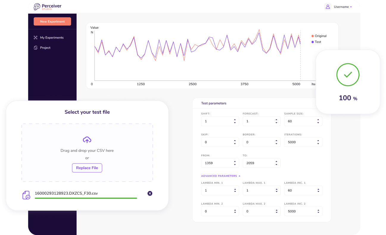
Based on this configuration file, Perceiver will run with a population size of 225,000 specimens. This number of candidate programs gets created every iteration and then the best ones are selected. The best solutions found are output alongside their fitness. In this demonstration, the best achieved fitness is 100%.

These results mean that with respect to the training set, this solution is arithmetically perfect. We can see that this is the mathematically correct solution for the sum of the first n numbers. It’s another format that has the addition of n squared over two plus n over 2 that is exactly the correct formula.

So far so good for the training set, but how did we do with the test set? For that result, we go to the output file for Perceiver. The first 49 records are the training results, with TRN in column D. As expected, they are 100% accurate.

But the interesting part is that the test results are also 100% accurate. We have the expected value in column F and the value predicted by the Perceiver model in column G. The model being used here is the formula for the sum of the first n numbers.

Perceiver Results

To emphasize the performance differential, we can review against the results from TensorFlow which are stored in a file. The output of the test set shows expected value and predicted value from TensorFlow. We then add another column: Perceiver predicted value. What we find is that Perceiver produces 100% mathematically accurate results even for variables that are out of the range for which the data was trained.

Something else to note is that Perceiver produces accurate results across the entire range with a relatively small number of records — just 49 in this case. It produces a compact, very easy to understand model that domain experts can actively digest and approve — whereas with TensorFlow, it’s only a graph of weights that is applied to the architecture that was used to predict. These are some of the advantages that we see in using Perceiver in cases like this against deep learning, a very commonly used AI solution.

Expected Results vs. Perceiver Results vs. TensorFlow Results